An implementation guide to Word2Vec using NumPy and Google Sheets!

Dec 5, 2018

Word2Vec is touted as one of the biggest, most recent breakthrough in the field of Natural Language Processing (NLP). The concept is simple, elegant and (relatively) easy to grasp. A quick Google search returns multiple results on how to use them with standard libraries such as Gensim and TensorFlow. Also, for the curious minds, check out the original implementation using C by Tomas Mikolov. The original paper can be found here too.

The main focus on this article is to present Word2Vec in detail. For that, I implemented Word2Vec on Python using NumPy (with much help from other tutorials) and also prepared a Google Sheet to showcase the calculations. Here are the links to the code and Google Sheet.

Intuition

The objective of Word2Vec is to generate vector representations of words that carry semantic meanings for further NLP tasks. Each word vector is typically several hundred dimensions and each unique word in the corpus is assigned a vector in the space. For example, the word “happy” can be represented as a vector of 4 dimensions [0.24, 0.45, 0.11, 0.49] and “sad” has a vector of [0.88, 0.78, 0.45, 0.91].

The transformation from words to vectors is also known as word embedding. The reason for this transformation is so that machine learning algorithm can perform linear algebra operations on numbers (in vectors) instead of words.

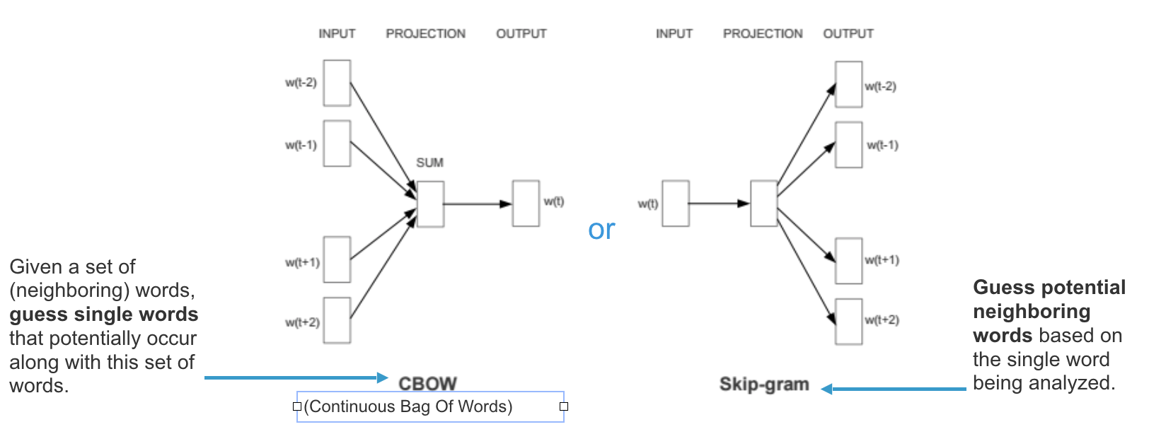
To implement Word2Vec, there are two flavors to choose from — Continuous Bag-Of-Words (CBOW) or continuous Skip-gram (SG). In short, CBOW attempts to guess the output (target word) from its neighbouring words (context words) whereas continuous Skip-Gram guesses the context words from a target word. Effectively, Word2Vec is based on distributional hypothesis where the context for each word is in its nearby words. Hence, by looking at its neighbouring words, we can attempt to predict the target word.

According to Mikolov (quoted in this article), here is the difference between Skip-gram and CBOW:

Skip-gram: works well with small amount of the training data, represents well even rare words or phrases

CBOW: several times faster to train than the skip-gram, slightly better accuracy for the frequent words

To elaborate further, since Skip-gram learns to predict the context words from a given word, in case where two words (one appearing infrequently and the other more frequently) are placed side-by-side, both will have the same treatment when it comes to minimising loss since each word will be treated as both the target word and context word. Comparing that to CBOW, the infrequent word will only be part of a collection of context words used to predict the target word. Therefore, the model will assign the infrequent word a low probability.

Implementation Process

In this article, we will be implementing the Skip-gram architecture. The content is broken down into the following parts for easy reading:

Data Preparation — Define corpus, clean, normalise and tokenise words
Hyperparameters — Learning rate, epochs, window size, embedding size
Generate Training Data — Build vocabulary, one-hot encoding for words, build dictionaries that map id to word and vice versa
Model Training — Pass encoded words through forward pass, calculate error rate, adjust weights using backpropagation and compute loss
Inference — Get word vector and find similar words
Further improvements — Speeding up training time with Skip-gram Negative Sampling (SGNS) and Hierarchical Softmax

1. Data Preparation

To begin, we start with the following corpus:

natural language processing and machine learning is fun and exciting

For simplicity, we have chosen a sentence without punctuation and capitalisation. Also, we did not remove stop words “and” and “is”.

In reality, text data are unstructured and can be “dirty”. Cleaning them will involve steps such as removing stop words, punctuations, convert text to lowercase (actually depends on your use-case), replacing digits, etc. KDnuggets has an excellent article on this process. Alternatively, Gensim also provides a function to perform simple text preprocessing using gensim.utils.simple_preprocess where it converts a document into a list of lowercase tokens, ignoring tokens that are too short or too long.

text = "natural language processing and machine learning is fun and exciting"

# Note the .lower() as upper and lowercase does not matter in our implementation
# [['natural', 'language', 'processing', 'and', 'machine', 'learning', 'is', 'fun', 'and', 'exciting']]
corpus = [[word.lower() for word in text.split()]]

After preprocessing, we then move on to tokenising the corpus. Here, we tokenise our corpus on whitespace and the result is a list of words:

[“natural”, “language”, “processing”, “ and”, “ machine”, “ learning”, “ is”, “ fun”, “and”, “ exciting”]

2. Hyperparameters

Before we jump into the actual implementation, let us define some of the hyperparameters we need later.

settings = {
	'window_size': 2	# context window +- center word
	'n': 10,		# dimensions of word embeddings, also refer to size of hidden layer
	'epochs': 50,		# number of training epochs
	'learning_rate': 0.01	# learning rate
}

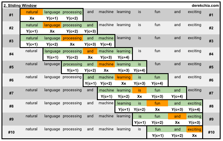
[window_size]: As mentioned above, context words are words that are neighbouring the target word. But how far or near should these words be in order to be considered neighbour? This is where we define the window_size to be 2 which means that words that are 2 to the left and right of the target words are considered context words. Referencing Figure 3 below, notice that each of the word in the corpus will be a target word as the window slides.

[n]: This is the dimension of the word embedding and it typically ranges from 100 to 300 depending on your vocabulary size. Dimension size beyond 300 tends to have diminishing benefit (see page 1538 Figure 2 (a)). Do note that the dimension is also the size of the hidden layer.

[epochs]: This is the number of training epochs. In each epoch, we cycle through all training samples.

[learning_rate]: The learning rate controls the amount of adjustment made to the weights with respect to the loss gradient.

3. Generate Training Data

In this section, our main objective is to turn our corpus into a one-hot encoded representation for the Word2Vec model to train on. From our corpus, Figure 4 zooms into each of the 10 windows (#1 to #10) as shown below. Each window consists of both the target word and its context words, highlighted in orange and green respectively.

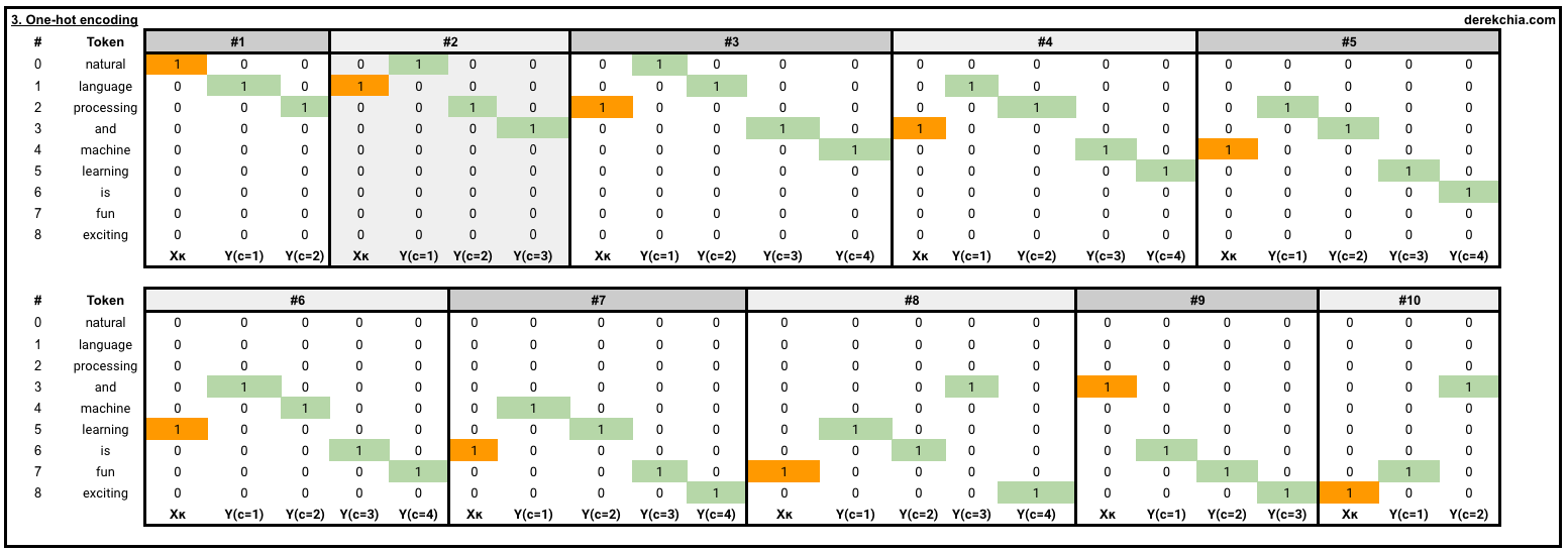
Example of the first and last element in the first and last training window is shown below:

1 [Target (natural)], [Context (language, processing)]

[list([1, 0, 0, 0, 0, 0, 0, 0, 0])

list([[0, 1, 0, 0, 0, 0, 0, 0, 0], [0, 0, 1, 0, 0, 0, 0, 0, 0]])]

2 to 9 removed

10 [Target (exciting)], [Context (fun, and)]

[list([0, 0, 0, 0, 0, 0, 0, 0, 1])

list([[0, 0, 0, 0, 0, 0, 0, 1, 0], [0, 0, 0, 1, 0, 0, 0, 0, 0]])]

To generate the one-hot training data, we first initialise the word2vec() object and then using the object w2v to call the function generate_training_data by passing settings and corpus as arguments.

# Initialise object
w2v = word2vec()
# Numpy ndarray with one-hot representation for [target_word, context_words]
training_data = w2v.generate_training_data(settings, corpus)

Inside the function generate_training_data, we performed the following operations:

self.v_count — Length of vocabulary (note that vocabulary refers to the number of unique words in the corpus)
self.words_list — List of words in vocabulary
self.word_index — Dictionary with each key as word in vocabulary and value as index
self.index_word — Dictionary with each key as index and value as word in vocabulary
for loop to append one-hot representation for each target and its context words to training_data using word2onehot function.

class word2vec():
  def __init__(self):
    self.n = settings['n']
    self.lr = settings['learning_rate']
    self.epochs = settings['epochs']
    self.window = settings['window_size']

  def generate_training_data(self, settings, corpus):
    # Find unique word counts using dictonary
    word_counts = defaultdict(int)
    for row in corpus:
      for word in row:
        word_counts[word] += 1
    ## How many unique words in vocab? 9
    self.v_count = len(word_counts.keys())
    # Generate Lookup Dictionaries (vocab)
    self.words_list = list(word_counts.keys())
    # Generate word:index
    self.word_index = dict((word, i) for i, word in enumerate(self.words_list))
    # Generate index:word
    self.index_word = dict((i, word) for i, word in enumerate(self.words_list))

    training_data = []
    # Cycle through each sentence in corpus
    for sentence in corpus:
      sent_len = len(sentence)
      # Cycle through each word in sentence
      for i, word in enumerate(sentence):
        # Convert target word to one-hot
        w_target = self.word2onehot(sentence[i])
        # Cycle through context window
        w_context = []
        # Note: window_size 2 will have range of 5 values
        for j in range(i - self.window, i + self.window+1):
          # Criteria for context word 
          # 1. Target word cannot be context word (j != i)
          # 2. Index must be greater or equal than 0 (j >= 0) - if not list index out of range
          # 3. Index must be less or equal than length of sentence (j <= sent_len-1) - if not list index out of range 
          if j != i and j <= sent_len-1 and j >= 0:
            # Append the one-hot representation of word to w_context
            w_context.append(self.word2onehot(sentence[j]))
            # print(sentence[i], sentence[j]) 
            # training_data contains a one-hot representation of the target word and context words
        training_data.append([w_target, w_context])
    return np.array(training_data)

  def word2onehot(self, word):
    # word_vec - initialise a blank vector
    word_vec = [0 for i in range(0, self.v_count)] # Alternative - np.zeros(self.v_count)
    # Get ID of word from word_index
    word_index = self.word_index[word]
    # Change value from 0 to 1 according to ID of the word
    word_vec[word_index] = 1
    return word_vec

4. Model Training

With our training_data, we are now ready to train our model. Training starts with w2v.train(training_data) where we pass in the training data and call the function train.

The Word2Vec model consists of 2 weight matrices (w1 and w2) and for demo purposes, we have initialised the values to a shape of (9x10) and (10x9) respectively. This facilitates the calculation of backpropagation error which will be covered later in the article. In the actual training, you should randomly initialise the weights (e.g. using np.random.uniform()). To do that, comment line 9 and 10 and uncomment line 11 and 12.

# Training
w2v.train(training_data)

class word2vec():
  def train(self, training_data):
  # Initialising weight matrices
  # Both s1 and s2 should be randomly initialised but for this demo, we pre-determine the arrays (getW1 and getW2)
  # getW1 - shape (9x10) and getW2 - shape (10x9)
  self.w1 = np.array(getW1)
  self.w2 = np.array(getW2)
  # self.w1 = np.random.uniform(-1, 1, (self.v_count, self.n))
  # self.w2 = np.random.uniform(-1, 1, (self.n, self.v_count))

Training — Forward Pass

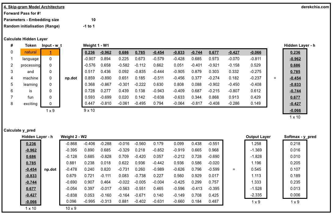
Next, we start training our first epoch using the first training example by passing in w_t which represents the one-hot vector for target word to the forward_pass function. In the forward_pass function, we perform a dot product between w1 and w_t to produce h (Line 24). Then, we perform another dot product using w2 and h to produce the output layer u (Line 26). Lastly, we run u through softmax to force each element to the range of 0 and 1 to give us the probabilities for prediction (Line 28) before returning the vector for prediction y_pred, hidden layer h and output layer u.

class word2vec():
  def train(self, training_data):
  ##Removed##
  
    # Cycle through each epoch
    for i in range(self.epochs):
      # Intialise loss to 0
      self.loss = 0

      # Cycle through each training sample
      # w_t = vector for target word, w_c = vectors for context words
      for w_t, w_c in training_data:
        # Forward pass - Pass in vector for target word (w_t) to get:
        # 1. predicted y using softmax (y_pred) 2. matrix of hidden layer (h) 3. output layer before softmax (u)
        y_pred, h, u = self.forward_pass(w_t)
        
        ##Removed##
        
  def forward_pass(self, x):
    # x is one-hot vector for target word, shape - 9x1
    # Run through first matrix (w1) to get hidden layer - 10x9 dot 9x1 gives us 10x1
    h = np.dot(self.w1.T, x)
    # Dot product hidden layer with second matrix (w2) - 9x10 dot 10x1 gives us 9x1
    u = np.dot(self.w2.T, h)
    # Run 1x9 through softmax to force each element to range of [0, 1] - 1x8
    y_c = self.softmax(u)
    return y_c, h, u
  
  def softmax(self, x):
    e_x = np.exp(x - np.max(x))
    return e_x / e_x.sum(axis=0)

I have attached some screenshots to show the calculation for the first training sample in the first window (#1) where the target word is ‘natural’ and context words are ‘language’ and ‘processing’. Feel free to look into the formula in the Google Sheet here.

Training — Error, Backpropagation and Loss

Error — With y_pred, h and u, we proceed to calculate the error for this particular set of target and context words. This is done by summing up the difference between y_pred and each of the context words in w_c.

Backpropagation — Next, we use the backpropagation function, backprop, to calculate the amount of adjustment we need to alter the weights using the function backprop by passing in error EI, hidden layer h and vector for target word w_t.

To update the weights, we multiply the weights to be adjusted (dl_dw1 and dl_dw2) with learning rate and then subtract it from the current weights (w1 and w2).

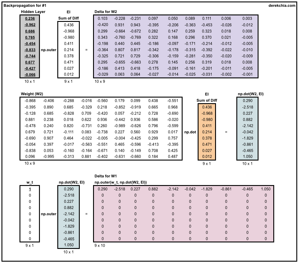
class word2vec():
  ##Removed##
  
  for i in range(self.epochs):
    self.loss = 0
    for w_t, w_c in training_data:
    ##Removed##
      
      # Calculate error
      # 1. For a target word, calculate difference between y_pred and each of the context words
      # 2. Sum up the differences using np.sum to give us the error for this particular target word
      EI = np.sum([np.subtract(y_pred, word) for word in w_c], axis=0)

      # Backpropagation
      # We use SGD to backpropagate errors - calculate loss on the output layer 
      self.backprop(EI, h, w_t)

      # Calculate loss
      # There are 2 parts to the loss function
      # Part 1: -ve sum of all the output +
      # Part 2: length of context words * log of sum for all elements (exponential-ed) in the output layer before softmax (u)
      # Note: word.index(1) returns the index in the context word vector with value 1
      # Note: u[word.index(1)] returns the value of the output layer before softmax
      self.loss += -np.sum([u[word.index(1)] for word in w_c]) + len(w_c) * np.log(np.sum(np.exp(u)))
    print('Epoch:', i, "Loss:", self.loss)

  def backprop(self, e, h, x):
    # https://docs.scipy.org/doc/numpy-1.15.1/reference/generated/numpy.outer.html
    # Column vector EI represents row-wise sum of prediction errors across each context word for the current center word
    # Going backwards, we need to take derivative of E with respect of w2
    # h - shape 10x1, e - shape 9x1, dl_dw2 - shape 10x9
    dl_dw2 = np.outer(h, e)
    # x - shape 1x8, w2 - 5x8, e.T - 8x1
    # x - 1x8, np.dot() - 5x1, dl_dw1 - 8x5
    dl_dw1 = np.outer(x, np.dot(self.w2, e.T))
    # Update weights
    self.w1 = self.w1 - (self.lr * dl_dw1)
    self.w2 = self.w2 - (self.lr * dl_dw2)

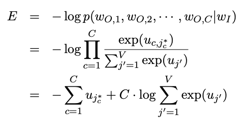
Loss — Lastly, we compute the overall loss after finishing each training sample according to the loss function. Take note that the loss function comprises of 2 parts. The first part is the negative of the sum for all the elements in the output layer (before softmax). The second part takes the number of the context words and multiplies the log of sum for all elements (after exponential) in the output layer.

5. Inferencing

Now that we have completed training for 50 epochs, both weights (w1 and w2) are now ready to perform inference.

Getting Vector for a Word

With a trained set of weights, the first thing we can do is to look at the word vector for a word in the vocabulary. We can simply do this by looking up the index of the word against the trained weight (w1). In the following example, we look up the vector for the word “machine”.

# Get vector for word
vec = w2v.word_vec("machine")

class word2vec():
  ## Removed ##
  
  # Get vector from word
  def word_vec(self, word):
    w_index = self.word_index[word]
    v_w = self.w1[w_index]
    return v_w

Find similar words

Another thing we can do is to find similar words. Even though our vocabulary is small, we can still implement the function vec_sim by computing the cosine similarity between words.

# Find similar words
w2v.vec_sim("machine", 3)

class word2vec():
  ## Removed##
  
  # Input vector, returns nearest word(s)
  def vec_sim(self, word, top_n):
    v_w1 = self.word_vec(word)
    word_sim = {}

    for i in range(self.v_count):
      # Find the similary score for each word in vocab
      v_w2 = self.w1[i]
      theta_sum = np.dot(v_w1, v_w2)
      theta_den = np.linalg.norm(v_w1) * np.linalg.norm(v_w2)
      theta = theta_sum / theta_den

      word = self.index_word[i]
      word_sim[word] = theta

    words_sorted = sorted(word_sim.items(), key=lambda kv: kv[1], reverse=True)

    for word, sim in words_sorted[:top_n]:
      print(word, sim)

$ w2v.vec_sim(“machine”, 3)

machine 1.0

fun 0.6223490454018772

and 0.5190154215400249

6. Further improvements

If you are still reading the article, well done and thank you! But this is not the end. As you might have noticed in the backpropagation step above, we are required to adjust the weights for all other words that were not involved in the training sample. This process can take up a long time if the size of your vocabulary is large (e.g. tens of thousands).

To solve this, below are the two features in Word2Vec you can implement to speed things up:

Skip-gram Negative Sampling (SGNS) helps to speed up training time and improve quality of resulting word vectors. This is done by training the network to only modify a small percentage of the weights rather than all of them. Recall in our example above, we update the weights for every other word and this can take a very long time if the vocab size is large. With SGNS, we only need to update the weights for the target word and a small number (e.g. 5 to 20) of random ‘negative’ words.
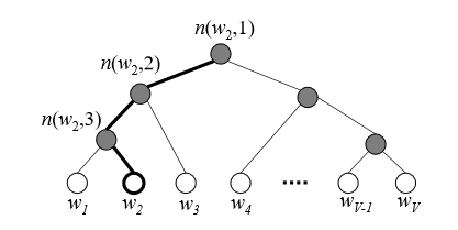
Hierarchical Softmax is also another trick to speed up training time replacing the original softmax. The main idea is that instead of evaluating all the output nodes to obtain the probability distribution, we only need to evaluate about log (based 2) of it. It uses a binary tree (Huffman coding tree) representation where the nodes in the output layer are represented as leaves and its nodes are represented in relative probabilities to its child nodes.

Beyond that, why not try tweaking the code to implement the Continuous Bag-of-Words (CBOW) architecture? 😃

Conclusion

This article is an introduction to Word2Vec and into the world of word embedding. It is also worth noting that there are pre-trained embeddings available such as GloVe, fastText and ELMo where you can download and use directly. There are also extensions of Word2Vec such as Doc2Vec and the most recent Code2Vec where documents and codes are turned into vectors. 😉

Lastly, I want to thank to Ren Jie Tan, Raimi and Yuxin for taking time to comment and read the drafts of this. 💪